Support Vector Machine
Regression
Support Vector Machines are very specific class
of algorithms, characterized by usage of kernels, absence of local minima,
sparseness of the solution and capacity control obtained by acting on the
margin, or on number of support vectors, etc.
They were invented by Vladimir Vapnik and his
co-workers, and first introduced at the Computational Learning Theory (COLT)
1992 conference with the paper. All these nice features however were already
present in machine learning since 1960’s: large margin hyper planes usage of
kernels, geometrical interpretation of kernels as inner products in a feature
space. Similar optimization techniques were used in pattern recognition and
sparsness techniques were widely discussed. Usage of slack variables to
overcome noise in the data and non - separability was also introduced in 1960s.
However it was not until 1992 that all these features were put together to form
the maximal margin classifier, the basic Support Vector Machine,
and not until 1995 that the soft margin version was introduced.
Support Vector Machine can be applied not only to
classification problems but also to the case of regression. Still it contains
all the main features that characterize maximum margin algorithm: a non-linear function
is leaned by linear learning machine mapping into high dimensional kernel
induced feature space. The capacity of the system is controlled by parameters
that do not depend on the dimensionality of feature space.
In the same way as with classification approach
there is motivation to seek and optimize the generalization bounds given for
regression. They relied on defining the loss function that ignores errors,
which are situated within the certain distance of the true value. This type of
function is often called – epsilon intensive – loss function. The figure below
shows an example of one-dimensional linear regression function with – epsilon
intensive – band. The variables measure the cost of the errors on the training
points. These are zero for all points that are inside the band.
Figure 1
One-dimensional linear regression with epsilon intensive band.
Another picture shows a similar situation but
for non-linear regression case.

Figure 2.
Non-linear regression function.
One of the most important ideas in Support
Vector Classification and Regression cases is that
presenting the solution by means of small subset of training points gives
enormous computational advantages. Using the epsilon intensive loss function we
ensure existence of the global minimum and at the same time optimization of
reliable generalization bound. 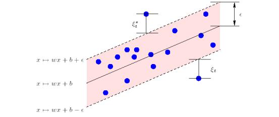
Figure 3.
Detailed picture of epsilon band with slack variables and selected data points
In SVM
regression, the input is first mapped onto a m-dimensional
feature space using some fixed (nonlinear) mapping, and then a linear model is
constructed in this feature space. Using mathematical notation, the linear
model (in the feature space)
is first mapped onto a m-dimensional
feature space using some fixed (nonlinear) mapping, and then a linear model is
constructed in this feature space. Using mathematical notation, the linear
model (in the feature space)  is given by
where  denotes a set of nonlinear transformations, and b is the “bias” term. Often the data are
assumed to be zero mean (this can be achieved by preprocessing), so the bias
term is dropped.
denotes a set of nonlinear transformations, and b is the “bias” term. Often the data are
assumed to be zero mean (this can be achieved by preprocessing), so the bias
term is dropped.
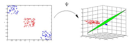
Figure 4. Non-linear mapping of input examples into
high dimensional feature space. (Classification case, however the same stands
for regression as well).
The quality of
estimation is measured by the loss function . SVM regression uses a new type of loss function called
  -insensitive loss function proposed by Vapnik:
The empirical risk is:
SVM regression
performs linear regression in the high-dimension feature space using  -insensitive loss and, at the same time, tries to reduce
model complexity by minimizing
-insensitive loss and, at the same time, tries to reduce
model complexity by minimizing  . This can be described by introducing (non-negative) slack
variables
. This can be described by introducing (non-negative) slack
variables
 , to measure the deviation of training samples outside
  -insensitive zone. Thus SVM regression is formulated as
minimization of the following functional:
-insensitive zone. Thus SVM regression is formulated as
minimization of the following functional:
min 
s.t. 
This optimization problem can
transformed into the dual problem and its solution is given by
 s.t.
s.t.  ,
, ,
,
where  is the number of Support Vectors (SVs) and the kernel
function
is the number of Support Vectors (SVs) and the kernel
function
It is well
known that SVM generalization performance (estimation accuracy) depends on a
good setting of meta-parameters parameters
C,  and the kernel
parameters. The problem of optimal parameter selection is further complicated
by the fact that SVM model complexity (and hence its generalization
performance) depends on all three parameters. Existing software implementations
of SVM regression usually treat SVM meta-parameters as user-defined inputs.
Selecting a particular kernel type and kernel function parameters is usually
based on application-domain knowledge and also should reflect distribution of
input (x) values of the training
data.
and the kernel
parameters. The problem of optimal parameter selection is further complicated
by the fact that SVM model complexity (and hence its generalization
performance) depends on all three parameters. Existing software implementations
of SVM regression usually treat SVM meta-parameters as user-defined inputs.
Selecting a particular kernel type and kernel function parameters is usually
based on application-domain knowledge and also should reflect distribution of
input (x) values of the training
data.
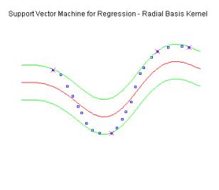
Figure 5. Performance of Support Vector Machine in
regression case. The epsilon boundaries are given with the green lines. Blue
points represent data instances.
Parameter C determines the trade off between the
model complexity (flatness) and the degree to which deviations larger than  are tolerated in
optimization formulation for example, if C
is too large (infinity), then the objective is to minimize the empirical risk
only, without regard to model complexity part in the optimization formulation.
are tolerated in
optimization formulation for example, if C
is too large (infinity), then the objective is to minimize the empirical risk
only, without regard to model complexity part in the optimization formulation.
Parameter  controls the width of the
  -insensitive zone, used to fit the training data. The value
of
-insensitive zone, used to fit the training data. The value
of  can affect the number of support vectors used to construct
the regression function. The bigger
can affect the number of support vectors used to construct
the regression function. The bigger  , the fewer support vectors are selected. On the other hand,
bigger
, the fewer support vectors are selected. On the other hand,
bigger  -values results in more ‘flat’ estimates. Hence, both C and
  -values affect model complexity (but in a different way).
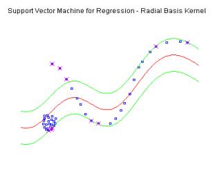
Figure 6.
Performance of Support Vector Machine in regression case. The epsilon
boundaries are given with the green lines. Blue points represent data
instances.
(Additional instances are introduced in this case and
after being supplied to the model are inside epsilon band. The regression
function has changed. However this makes some points that were initially inside
the interval to be misclassified.)
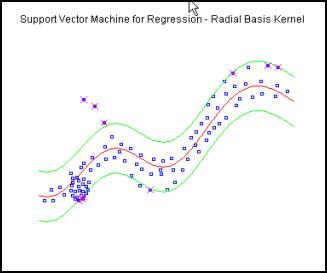
Figure 7.
Performance of Support Vector Machine in regression case. The epsilon
boundaries are given with the green lines. Blue points represent data
instances.
(Introducing new data instances
that are located inside the epsilon band, do not influence the structure of the
model. It can be seen that regression function has not changed at all.)
One of the advantages of Support Vector
Machine, and Support Vector Regression as the part of it,
is that it can be used to avoid difficulties of using linear functions in the
high dimensional feature space and optimization problem is transformed into
dual convex quadratic programmes. In regression case the loss function is used
to penalize errors that are grater than threshold -  . Such loss functions usually lead to the sparse
representation of the decision rule, giving significant algorithmic and
representational advantages.
. Such loss functions usually lead to the sparse
representation of the decision rule, giving significant algorithmic and
representational advantages.
References
O. Chapelle and V. Vapnik, Model
Selection for Support Vector Machines. In Advances in Neural Information Processing Systems, Vol
12, (1999)
V. Cherkassky and Y. Ma, Selecting of
the Loss Function for Robust Linear Regression, Neural computation 2002.
V. Cherkassky and F. Mulier, Learning
from Data: Concepts, Theory, and Methods. (John Wiley & Sons, 1998)
Y.B.
Dibike, S. Velickov, D.P. Solomatine. Support vector machines: review and
applications in civil engineering. In: AI methods in Civil Engineering
Applications (O. Schleider, A. Zijderveld, eds). Cottbus, 2000, p.45-58
Y.B.
Dibike, S. Velickov, D.P. Solomatine. and M. B. Abbott Model induction with
support vector machines: introduction and applications. Journal of Computing in
Civil Engineering, American Society of Civil Engineers (ASCE), vol. 15, No.3,
2001, pp. 208-216
A. Smola
and B. Schölkopf. A Tutorial on Support Vector Regression. NeuroCOLT
Technical Report NC-TR-98-030, Royal Holloway College, University of London,
UK, 1998
T. Yoshioka and S. Ishii, Fast
Gaussian process regression using representative data,
International Joint Conference on Neural Networks 1, 132-137, 2001.
Useful links:
1.
Kernels-Machines.org Ultimate
resource in machine learning.
2.
Intelligent Data
Analysis. GMD.
3.
Isabelle
Guyon's SVM application list. Berkeley.
4.
COLT Group.
Royal Holloway College.
5.
Machine Learning
Group. ANU Canberra.
6.
Gaussian Processes
Homepage. Toronto.
7.
Support Vector
Machines. Royal Holloway College.
8.
SVM Book Site.
Nello Cristianini and John Shawe-Taylor.
9.
Learning Theory
Website. COLT.